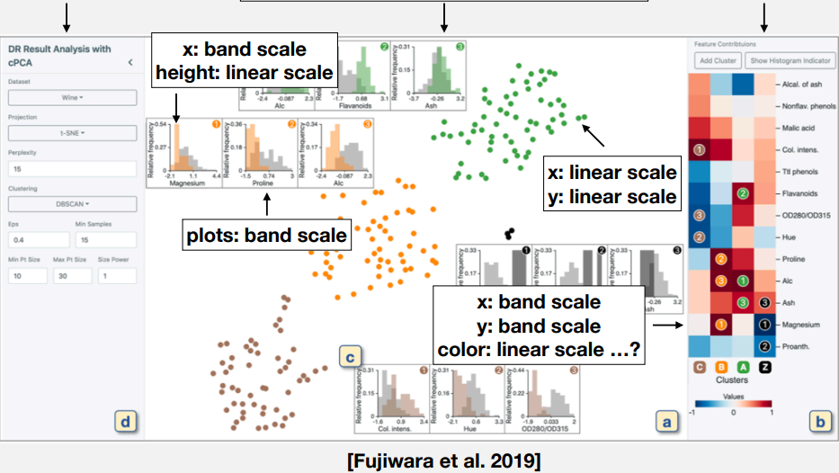
Visualization design: more than just a typology of visualizations
Space of visualizations
Designing with Data and Graphics
We will take a more granular approach to authoring visualizations
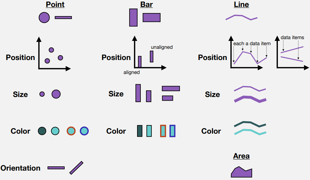
Each data item is encoded by a graphical mark
How we draw the mark is dependent on the data item’s attributes, or fields.
A structured approach to graphics creation helps us understand the design space
Declarative Approach to Design
Choose a mark
For each attribute:
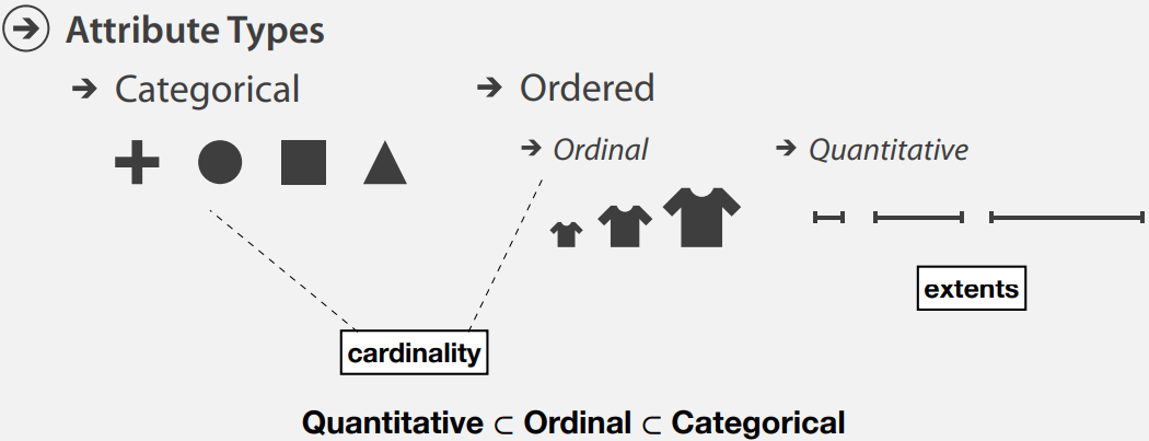
• Determine the attribute’s type
• Choose a visual channel
• Choose a mapping: from data domain to visual range
• … draw it!
• (there are some variations to this approach)
Graphical Marks, Visual Channels
Data: Attributes
Starting from data, how do we go to graphics?
First, need to determine a data item’s attribute.
Scales
Next: we choose a mapping from data domain, to visual range. A scale.
We distinguish scales via data attributes. Data domain or visual range can be categorical, ordinal, or quantitative.
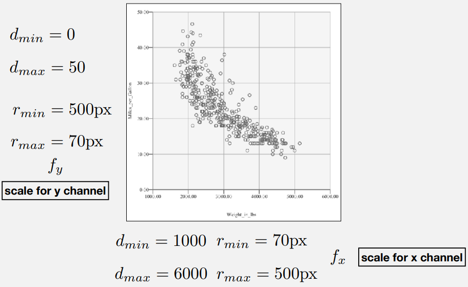
Quantitative: Quantitative Linear Scale
Domain and range are both quantitative. We first consider a linear scale.
Mathematical preliminaries:
Assume data domain has a minimum and maximum value \[ d_{min} \rightarrow d_{max}\]
Assume data range has a minimum and maximum value \[ r_{min} \rightarrow r_{max}\]
Quantitative: Quantitative Linear Scale
We seek a linear function such that: \[ f(d_{min}) = r_{min}\] and \[ f(d_{max}) = r_{max}\]
Quantitative: Quantitative Linear Scale
Two step process:
Normalize data in domain: \[
\alpha(d) = \frac{d - d_{min}}{d_{max} - d_{min}}
\]
Linear interpolation in the range: \[
f(\alpha(d)) = (1 - \alpha(d)) . r_{min} + \alpha(d) . r_{max}
\]
Linear Scale example
Other Quantitative Scales
Can be used for different functions, e.g. quadratic, square root, etc..
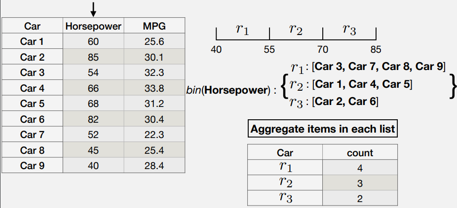
Our data domain is quantitative, our visual range is discrete - and in particular, ordered. \[ d_{min} \rightarrow d_{max} \\
R = [r_1, r_2, \dots, r_n]
\]
Common assumption: range is uniformly divided by the domain. \[ f(\alpha(d)) = r_i \text{ Where } i = 1 + \lfloor n.\alpha_d \rfloor \]
Special Case: Binning Transformation
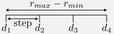
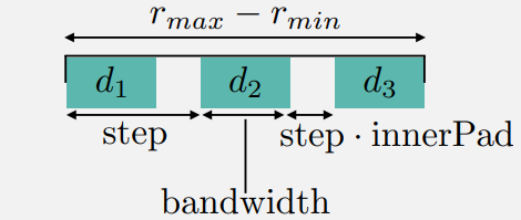
Ordinal: Quantitative Point Scale
Our data domain is ordinal, our visual range is quantitative. \[
D = [d_1, d_2, \dots, d_m] \text{ and } r_{min} \rightarrow r_{max}
\]
It is also common to introduce padding at the beginning and end.
\[
f(d_i) = r_{min} + (i-1).step
\]
Used for: bar marks, group transformations.
Example
Recap: A Recipe for Authoring Visualizations
Ingredients: • Identify data items.
• Select data attributes.
• Determine a type for each attribute.
• Determine a graphical mark for an item.
• Select a visual channel for each attribute.
• Select a scale for each channel.